9. Regions and a tour of the reasoning layer
In this lesson: systems that switch behavior at a threshold, and a quick tour of the analysis tools built on top of the simulator. This is your map to the rest of the library.
Part A — Regions: piecewise systems
Real systems change their rules at thresholds. A tank overflows once it's full — beyond the brim, the physics is different (excess spills; the level holds at the top). The library models this with operating regions: named subsets of constraints that are active in different parts of state space, with guarded transitions between them.
Here's the bathtub upgraded so that reaching the brim while still filling crosses into a steady-overflow region:
import qrlib as qr
from qrlib import Qdir, TimeTag

m = qr.Model("overflow bathtub")
m.variable("amount",  landmarks=("0", "FULL"))
m.variable("level",   landmarks=("0", "TOP"))
m.variable("outflow", landmarks=("0", "OMAX"))
m.variable("inflow",  landmarks=("0", "IF"))
m.variable("netflow", landmarks=("0",), unbounded=True)

c_al  = m.constrain(qr.MPlus("amount", "level",  cvals=(("0", "0"), ("FULL", "TOP"))))
c_lo  = m.constrain(qr.MPlus("level",  "outflow", cvals=(("0", "0"), ("TOP", "OMAX"))))
c_add = m.constrain(qr.Add("netflow", "outflow", "inflow"))
c_der = m.constrain(qr.Deriv("amount", "netflow"))
c_inf = m.constrain(qr.Constant("inflow"))
c_amt = m.constrain(qr.Constant("amount"))          # amount held while overflowing

# two regions: while filling, and while overflowing
m.region("filling",     constraints=(c_al, c_lo, c_add, c_der, c_inf))
m.region("overflowing", constraints=(c_al, c_lo, c_add, c_inf, c_amt))

# cross when the tub is full *and* still gaining water
m.transition("filling", "overflowing",
             when=(("amount", "==", "FULL"), ("netflow", ">", "0")))

initial = m.state(time=TimeTag.POINT,
                  amount=("0", Qdir.INC), level=("0", Qdir.INC),
                  outflow=("0", Qdir.INC), inflow=("IF", Qdir.STD),
                  netflow=(("0", "+inf"), Qdir.DEC))

result = qr.qsim(m, initial)
print(result.stats["region_crossings"])   # 1
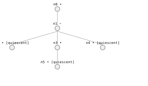
One of the behaviors now crosses regions — you can see it in the results:
for b in result.behaviors():
    print(b.terminal.value, b.regions)
quiescent   ('filling', 'filling', 'filling')                  # settles below the brim
quiescent   ('filling', 'filling', 'filling', 'overflowing')   # fills, then overflows steadily
quiescent   ('filling', 'filling', 'filling')                  # settles exactly at the brim
The middle behavior fills, hits FULL while still gaining, crosses into
the overflow region, and there reaches a new steady state (spilling the excess
at the brim). At the crossing, magnitudes carry over continuously and only the
directions re-derive under the new region's rules — that's how the tub goes
from "rising" to "held at the top."
Part B — A tour of the reasoning layer
Everything so far produces or refines a behavior graph. The library also reasons about those graphs. Here are the main tools, each a few lines. Rebuild the plain bathtub from Lessons 3–4 under unambiguous names:
plain = qr.Model("bathtub")
plain.variable("amount", landmarks=("0", "FULL"))
plain.variable("level", landmarks=("0", "TOP"))
plain.variable("outflow", landmarks=("0", "OMAX"))
plain.variable("inflow", landmarks=("0", "IF"))
plain.variable("netflow", landmarks=("0",), unbounded=True)
plain.constrain(qr.MPlus("amount", "level",
                        cvals=(("0", "0"), ("FULL", "TOP"))))
plain.constrain(qr.MPlus("level", "outflow",
                        cvals=(("0", "0"), ("TOP", "OMAX"))))
plain.constrain(qr.Add("netflow", "outflow", "inflow"))
plain.constrain(qr.Deriv("amount", "netflow"))
plain.constrain(qr.Constant("inflow"))
plain_initial = plain.state(
    time=TimeTag.POINT,
    amount=("0", Qdir.INC),
    level=("0", Qdir.INC),
    outflow=("0", Qdir.INC),
    inflow=("IF", Qdir.STD),
    netflow=(("0", "+inf"), Qdir.DEC),
)
plain_result = qr.qsim(plain, plain_initial)
What causes what — analysis.causal
Derives the causal structure from the constraints alone (no simulation):
from qrlib.analysis import causal
order = causal.causal_order(plain)
print(order.exogenous)        # ('inflow',)   — the driving input
print(order.state_variables)  # ('amount',)   — the system's memory
print(causal.narrate_causes(order))
What-if questions — analysis.compare
Comparative analysis: perturb a parameter and get the sign of change of every quantity at equilibrium.
from qrlib.analysis import compare
change = compare.compare(plain, {"inflow": +1})   # turn the tap up
print({k: v.symbol for k, v in change.changes.items()})
# {'amount': '↑', 'level': '↑', 'outflow': '↑', 'inflow': '↑', 'netflow': '·'}
Read it: raise the inflow and the equilibrium amount, level, and outflow all rise, while the net flow stays zero (it's an equilibrium). Derived purely by sign propagation — no numbers.
Checking and focusing behaviors — qrlib.guide
First classify the complete, unguided graph. This is temporal-logic model checking:
from qrlib import guide
from qrlib.guide import G, mag

# "the amount stays below FULL forever" (a safety property)
spec = G(mag("amount", "<", "FULL"))
checked = guide.classify(plain_result, spec)
print(len(checked.satisfied), len(checked.violated), checked.universal)
# 1 2 False
One predicted behavior satisfies the property and two violate it, so it is not universal over the original model. Guided simulation instead treats the formula as an additional trajectory constraint and avoids expanding bad prefixes:
focused = guide.guided(plain, plain_initial, spec)
print(len(focused.satisfied), focused.result.stats["spec_filtered"])
# 1 2
The focused graph still covers every real behavior that satisfies spec.
Finding a satisfying qualitative path does not prove that path exists.
Which part is broken — qrlib.diagnosis
Model-based diagnosis: give components fault modes and observations, and get
minimal explanations. Here a sensor expected to stay at HIGH is observed
stuck at zero:
from qrlib import diagnosis
from qrlib import Landmark
from qrlib.bridge.abstraction import abstract_trajectory

sensor_model = qr.Model("sensor")
sensor_model.variable(
    "reading",
    landmarks=(Landmark("0", 0.0), Landmark("HIGH", 1.0)),
)
sensor = diagnosis.Component("sensor", modes={
    "ok": (qr.Constant("reading"), qr.At("reading", "HIGH")),
    "stuck_low": (qr.Constant("reading"), qr.At("reading", "0")),
})
observed = abstract_trajectory([[0.0]] * 20, sensor_model)
observed_initial = sensor_model.state(reading=("0", Qdir.STD))
diagnosed = diagnosis.diagnose(
    sensor_model, [sensor], observed, initial=observed_initial
)
print(diagnosed.fault_detected)                       # True
print(dict(diagnosed.diagnoses[0].modes))             # {'sensor': 'stuck_low'}
The normal mode is refuted because its At(reading, HIGH) operating point
cannot cover the observation. Diagnosis searches fault sets in increasing
cardinality and uses the coverage oracle as its consistency check.
Where to go next
You now have the core mental model. The advanced tutorial track develops the remaining public surfaces with runnable examples:
| Want to… | Reach for |
|---|---|
| Make models/results portable and replayable | Lesson 10 |
| Integrate hybrid numeric trajectories | Lesson 11 |
| Learn structure and diagnose faults | Lesson 12 |
| Envision and analyze whole behavior spaces | Lesson 13 |
| Author components and scale execution | Lesson 14 |
| Put the complete host-facing workflow together | Lesson 15 |
For the design behind it all, see the top-level docs/: architecture.md
(how the pieces fit), qsim.md (the engine), host-integration.md (using the
library from a larger system), and literature-survey.md (where these ideas
come from).
Exercises
- In the region model, change the crossing guard to fire on
amount == FULLalone (drop thenetflow > 0condition). Does the behavior that settles exactly at the brim now wrongly cross into overflow? Why is the extra guard important? - Use
compare.compareto predict what happens to the equilibrium level if you made the drain more efficient (imagine anoutflowthat rises faster with level). Sketch how you'd encode that perturbation. - Run both the
classifyandguidedexamples. Explain why the former says the property is not universal while the latter produces only one satisfying behavior.
That's the core track. You can now describe a system qualitatively, simulate every behavior it admits, tame spurious clutter soundly, add numbers for tighter bounds, and reason about causes, faults, and what-ifs. Continue with Lesson 10 for the complete public-library tour.