Extended Kalman filter for a Differential Drive Robot

Introduction to Extended Kalman Filters

Like the Kalman filter, the Extended Kalman Filter (EKF) operates on Gaussian distributions. However, where the Kalman filter requires its action and sensor models to be linear systems, the EKF can use models based on non-linear systems. The motion model for a differential drive robot defined in part one of this series is an example of a non-linear system.

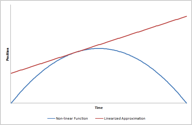
The EKF linearizes the non-linear system around the current state. The graph below demonstrates this process.

The blue line represents a non-linear path over time. The red line represents a linearization of the non-linear path at a single moment in time. The error between the non-linear function and the linearized approximation grows as the distance from the linearized point grows.

EKF uses a state type X and an action type U. The action model transition function defines x_posterior = g(x_prior, u_current). This non-linear function is linearized by taking the gradient, or Jacobian, of this system. If the prior has a non-zero covariance, then that error is shaped by the Jacobian of g with respect to X. If the action has a non-zero covariance, then the action covaraince is shaped by the Jacobian of X with respect to U and added to the posterior covariance.

It is very common for the action to be treated as a perfectly known value and a constant error value is relied upon to expand the probable range of the posterior.

Action Update

As in the Kalman filter, each point in the prior state belief is transformed by the action model. Again, this is done in a closed form. The prior is shaped by the gradient (Jacobian) of the transition function with respect to the state at the mean of the state prior and action. Process noise is added to the resulting posterior. If the action is provided as a distribution, then the gradient of the transition function with respect to the action is used to tranform the action mean into action noise which is also added to the posterior.

The gradient with respect to the state is:

G_X = [
    ∂x/∂x  ∂x/∂y  ∂x/∂θ
    ∂y/∂x  ∂y/∂y  ∂y/∂θ
    ∂θ/∂x  ∂θ/∂y  ∂θ/∂θ
]

The gradient with respect to the action is:

G_U = [
    ∂x/∂V_L  ∂x/∂V_R  ∂x/∂t
    ∂y/∂V_L  ∂y/∂V_R  ∂y/∂t
    ∂θ/∂V_L  ∂θ/∂V_R  ∂t/∂t
]

DifferentialDriveAction model provides the left and right velocities and the time period over which to apply the control. Implementations for these Jacobians are provided by DifferentialDriveActionModel. The following Silverlight app shows the state Jacobian in red and the action Jacobian in blue (note that for simplicity of visualization, the heading component is not displayed). The state transtion component mostly affects how far to the left and right the robot's path may vary. The action transition affects only the distance traveled by the robot. The action Jacobian is singular. It projects any action error onto a line along the robot's direction of travel.

ExtendedKalmanFilter requires its action model to be an ExtendedKalmanActionModel. ExtendedKalmanActionModel defines the methods that provide the state and action Jacobians. DDActionModel implements this interface with the actual implementations for the Jacobian function derived from DifferentialDriveActionModel. The code for the EKF action model follows.

public class DDActionModel :
    DifferentialDriveActionModel,
    ExtendedKalmanActionModel<DifferentialDriveAction, Pose> {

    public Matrix R { get; set; }

    public Pose GetMean(DifferentialDriveAction action, Pose state) {
        return this.GetNextState(action, state);
    }

    public Matrix GetError(DifferentialDriveAction action, Pose state) {
        return action.Time * R;
    }

    public override RandomDistribution<Pose> ConditionBy(DifferentialDriveAction action, Pose state) {
        return new GaussianMoment<Pose>(GetMean(action, state), GetError(action, state));
    }
}

The code to set up the filter is very similar to that of the Kalman filter.

DDActionModel actionModel = new DDActionModel();
actionModel.AxleLength = 5;
actionModel.R = new Matrix(3, 3, 0.1, 0, 0, 0, 0.1, 0, 0, 0, 0.06);
ExtendedKalmanFilter<Pose, DifferentialDriveAction, PoseObservation> filter =
    new ExtendedKalmanFilter<Pose, DifferentialDriveAction, PoseObservation>();
filter.Belief = new GaussianMoment<Pose>(
    new Pose(200, 50, 0),
    new Matrix(3, 3, 10, 0, 0, 0, 10, 0, 0, 0, 0.01)
);
filter.ActionModel = actionModel;

The code to update the belief is simpler than that of the Kalman filter.

DifferentialDriveAction u = new DifferentialDriveAction(data.Vl, data.Vr, data.t);
filter.UpdateBeliefWithAction(u);

Sensor Update

The sensor update uses the same linearization technique in the EKF. However, for this tutorial, we will use the same sensor model as we did with the Kalman filter.

The code for the EKF sensor model follows. The sensor update code is exactly the same as the Kalman filter.

public class DDSensorModel
    :   KalmanSensorModel<PoseObservation, Pose>,
        ExtendedKalmanSensorModel<PoseObservation, Pose> {
    public DDSensorModel() { this.C = Matrix.CreateIdentity(3); }
    public Matrix GetJacobian(PoseObservation observation) { return C; }
}

DDSensorModel sensorModel = new DDSensorModel();
sensorModel.Q = new Matrix(3, 3,
    100, 0, 0,
    0, 100, 0,
    0, 0, 1);
filter.SensorModel = sensorModel;

PoseObservation z = GetObservation();
filter.UpdateBeliefWithObservation(z);

Extended Kalman filter for a Differential Drive Robot

Introduction to Extended Kalman Filters

Relationship to Kalman Filter

Action Update

Sensor Update

Differential Drive Tutorial Series: