Bayes Filters for a Differential Drive Robot
Introduction
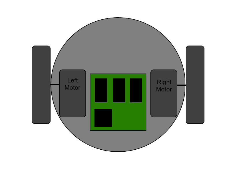
A common design for robot locomotion is the differential drive. The differential
drive consists of two wheels independently controlled by two motors. Such an arrangement
allows the robot to move forward and backwards, turn in place, and turn while moving.
This tutorial will show you how to build an action model for a differential drive
robot, and adapt that action model to different Bayes filters used to track
the robot's position and heading.
The Bayes Filter
The Bayes filter is a tool for state estimation. In this tutorial it will be used to track
the location and heading of a robot. The Bayes filter maintains a belief of probable poses of the
robot. This belief is updated through repeated applications of actions and observations.
Bayes filters use action models to describe how the belief should be updated by an action,
and sensor models to describe how the belief should be updated by an observation. Action
updates generally decrease the certainty of the state belief. Observation updates
generally increase the certainty of the state belief. There are several different types of Bayes
filters which use different representations and error models for the belief, action models,
and sensor models. This tutorial will look at tracking a robot's pose using the Kalman filter,
extended Kalman filter, unscented Kalman filter, and particle filter.
The interface
BayesFilter
defines the methods on a Bayes filter. BayesFilter is a generic defined with types <X, U, Z>. X is the type of the state
being estimated, U is the type of the action applied at a state, and Z is the observation type used to refine the state belief.
BayesFilter defines two methods:
- UpdateBeliefWithAction(U)
- Uses an action to transition the current state belief to a new state belief.
- UpdateBeliefWithObservation(Z)
- Updates the state belief with an observation.
Action Models Basics
Action models use an action and a start state to predict an expected end state. However,
since Bayes filters are based on probability, the action model actually has to
return a distribution of possible end states. Sometimes this is done by using
the expected state as a parameter in a distribution function. Other times this is
done calculating multiple expected end states using samples from an action distribution.
The action model can provide several sources for new possible states.
The state transition defined by the action model transforms all of the previous possible
states. This transform may not just shift the states in space, it may also change
the shape of the distribution. The action model may be able to operate on a distribution
of actions instead of a single know action. Having multiple actions will increase the range
of probable states. Lastly, the action model may introduce random noise to create new states.
The interface
ActionModel
defines the method needed for an action model. ActionModel is a generic defined with types <U, X>
Technically, action models are conditional distributions.
ActionModel only requires the subset of
ContinuousDistribution
needed by BayesFilter.
ActionModel defines the method:
- ConditionBy(U, X)
- Creates a distributions of possible states resulting from performing a specific action at a specific state.
Differential Drive Kinematics
We will assume that the robot has control over the velocity of its wheels. Given
two velocities for the wheels, the robot travels along a circular path with some
turn radius.
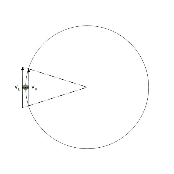
Let vL and vR be the left and right velocity
controls (in m/s). Let t be the time period over which the control is applied
(in s).
U = [ t, vL, vR]
We want to update the robot pose. The pose contains an x cooridinate a y coordinate and a heading θ.
X = [ x, y, θ]
We will defined an action model P(Xnext | Ut, Xprevious ).
This is the conditional probability of arriving at a state by performing an action at another state.
For now we will ignore the fact that the result is a distribution and calculate a single resulting state.
Let L be the axle length between the drive wheels.
The velocity of the robot, v, is calculated by taking the average of the two wheel velocities.
v = (vL + vR) / 2
Let R be the turn radius calculated by
R = v * (L / (vL - vR ))
R is negative if the robot is turning right and positive if the robot is turning left.
Let φ' be the angular velocity of the robot in radians per second.
φ' = (vL - vR) / L
Let R be the turn radius calculated by
R = v / φ'
R is negative if the robot is turning left and positive if the robot is turning right.
Xnext = [
xprev - R * sin(θprev) + R * sin(θprev + φ' * t)
yprev + R * cos(θprev) - R * cos(θprev + φ' * t)
θprev + φ' * t
]
DifferentialDriveActionModel
implements these equations as an
ActionModel.
DifferentialDriveActionModel operates on
DifferentialDriveAction
and Pose.
DifferentialDriveAction defines the left and right velocity controls and a time period.
Pose defines the x and y coordinates and heading of the robot.
Differential Drive Tutorial Series:
Copyright 2009 Cognitoware. All rights reserved.